How neural networks learn fits in one loop: the network makes a prediction, a loss function scores how wrong it was, backpropagation works out how much each weight contributed to the error, and gradient descent moves every weight a small step in the direction that reduces it. This guide does one training step by hand with real numbers, checks them with code, rewrites the step as a minimal PyTorch training loop, and then shows, with measured runs, what goes wrong in practice.
What "learning" means for a neural network
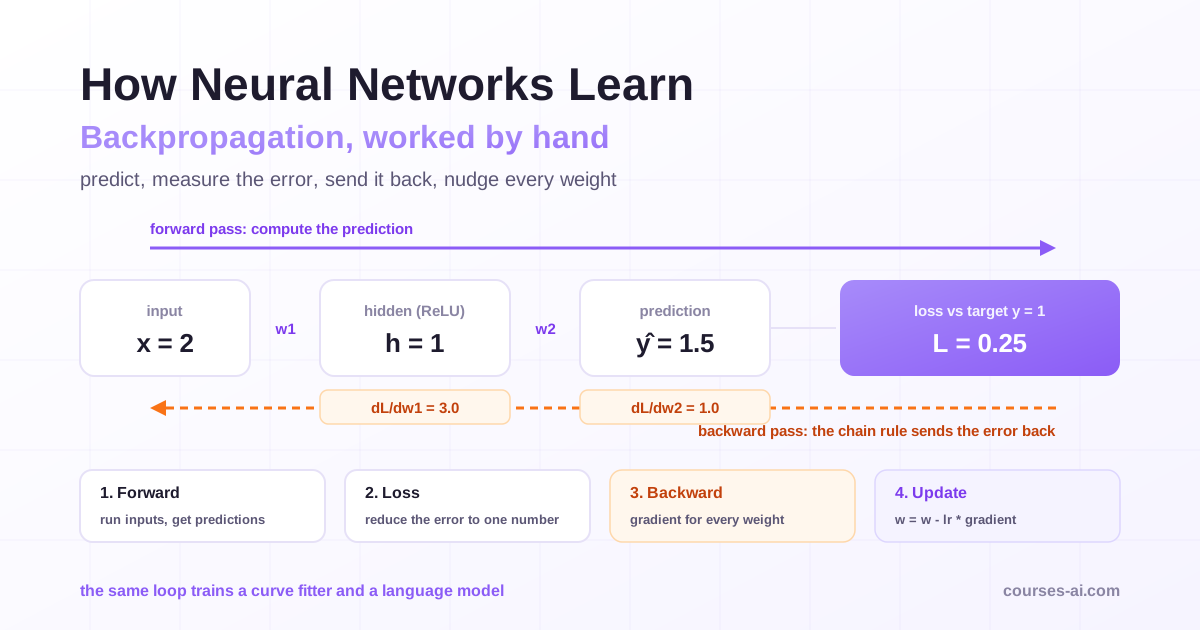
A neural network is a function with adjustable numbers inside it: weights and biases, the parameters. Training means searching for parameter values that make the outputs useful, and "useful" has to be written down as a single number the computer can minimize. That number is the loss. Every training step has four parts:
- Forward pass. Run the inputs through the network and get predictions.
- Loss. Compare predictions with targets and reduce the error to one number.
- Backward pass. Compute the gradient of the loss with respect to every parameter: how much the loss would change if that parameter moved slightly.
- Update. Move each parameter a small step against its gradient.
The terms get blurred, so be precise. As Goodfellow, Bengio and Courville put it in Deep Learning, chapter 6, "back-propagation refers only to the method for computing the gradient, while another algorithm, such as stochastic gradient descent, is used to perform learning using this gradient." Backpropagation is step 3, gradient descent is step 4, and they fail in different ways.
The same chapter traces the idea to control problems in the 1960s and 1970s, credits Werbos (1981) with proposing it for neural networks, and lists independent rediscoveries by LeCun (1985), Parker (1985) and Rumelhart, Hinton and Williams, whose paper Learning representations by back-propagating errors (Nature, 9 October 1986) is the best-known version. Its abstract states the key result: through the weight adjustments, internal "hidden" units "come to represent important features of the task domain". Nobody tells the hidden layers what to compute; the gradient does.
If you use LLMs through APIs you will rarely train a network, but this loop explains why fine-tuning can break a model and why every training config has a learning rate. Activation functions, initialization, the full training loop, CNNs and the Transformer are built up module by module, with PyTorch code, in Deep Learning and Neural Networks with PyTorch.
A worked example: one training step by hand
Take the smallest network with a hidden layer: one input, one hidden neuron with a ReLU activation, one output, four parameters.
z1    = w1 * x + b1          # hidden pre-activation
h     = relu(z1)             # hidden activation: max(0, z1)
y_hat = w2 * h + b2          # prediction
L     = (y_hat - y) ** 2     # squared-error loss
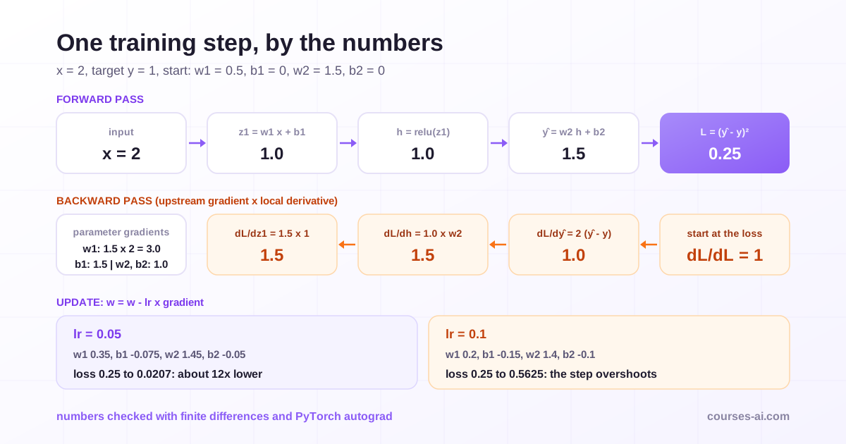
The training example is x = 2.0 with target y = 1.0. The starting parameters are w1 = 0.5, b1 = 0.0, w2 = 1.5, b2 = 0.0; in a real network they would be random, here they keep the arithmetic readable.
The forward pass
z1 = 0.5 * 2.0 + 0.0 = 1.0h = relu(1.0) = 1.0(positive, so it passes through)y_hat = 1.5 * 1.0 + 0.0 = 1.5L = (1.5 - 1.0)^2 = 0.25
The loss function
Squared error is the standard loss function for regression; classification and language models use cross-entropy, which measures how much probability the model gave the correct answer. The loss is the only definition of "good" the network ever sees: anything you care about that is not in it is not being optimized.
The backward pass: backpropagation explained one node at a time
Backpropagation starts at the loss and walks backward through the same computation. Each node multiplies the gradient arriving from the node after it (the upstream gradient) by its own local derivative:
- At the output:
dL/dy_hat = 2 * (y_hat - y) = 2 * 0.5 = 1.0 - Output parameters, where
y_hat = w2 * h + b2:dL/dw2 = 1.0 * h = 1.0anddL/db2 = 1.0 - Into the hidden layer:
dL/dh = 1.0 * w2 = 1.5 - Through the ReLU, whose derivative is 1 for positive inputs and 0 otherwise:
dL/dz1 = 1.5 * 1 = 1.5 - Hidden parameters, where
z1 = w1 * x + b1:dL/dw1 = 1.5 * x = 3.0anddL/db1 = 1.5
Two details matter. First, dL/dy_hat was computed once and reused for every parameter behind it, which is why backpropagation gets all gradients at a cost of the same order as the forward pass (in practice about twice its compute), instead of one pass per weight. Second, the gradient reaching w1 is a product: 2 * (y_hat - y) * w2 * relu'(z1) * x. Stack twenty layers and it becomes a product of dozens of factors, which is where vanishing and exploding gradients come from.
The update: gradient descent explained in one line
Gradient descent moves each parameter against its gradient, scaled by the learning rate: parameter = parameter - learning_rate * gradient. With a learning rate of 0.05:
w1 = 0.5 - 0.05 * 3.0 = 0.35b1 = 0.0 - 0.05 * 1.5 = -0.075w2 = 1.5 - 0.05 * 1.0 = 1.45b2 = 0.0 - 0.05 * 1.0 = -0.05
Run the forward pass again: z1 = 0.625, y_hat = 0.85625, and the loss drops from 0.25 to about 0.0207, twelve times smaller in one step.
Now use a learning rate of 0.1. The parameters become w1 = 0.2, b1 = -0.15, w2 = 1.4, b2 = -0.1, the prediction becomes 0.25, and the loss rises to 0.5625. Same gradient, worse result. The gradient is a local slope: it says which way is downhill here, not how far. A step that is too long jumps past the valley floor and up the other side.
To check a hand derivation, nudge each parameter by a tiny amount in both directions and measure the change in the loss. This finite-difference estimate is too slow to train with, but it is the standard test for a hand-written backward pass (PyTorch ships it as torch.autograd.gradcheck). Run in plain Python with a nudge of 1e-6, it returns 3.0, 1.5, 1.0 and 1.0, matching the chain rule above.
The same step in PyTorch
PyTorch's autograd records every operation in the forward pass and, when you call backward(), runs the chain rule in reverse exactly as we did:
import torch

x, y = torch.tensor(2.0), torch.tensor(1.0)
w1 = torch.tensor(0.5, requires_grad=True)
b1 = torch.tensor(0.0, requires_grad=True)
w2 = torch.tensor(1.5, requires_grad=True)
b2 = torch.tensor(0.0, requires_grad=True)

h = torch.relu(w1 * x + b1)
y_hat = w2 * h + b2
loss = (y_hat - y) ** 2
loss.backward()

print(loss.item())                                   # 0.25
print([p.grad.item() for p in (w1, b1, w2, b2)])     # [3.0, 1.5, 1.0, 1.0]
On PyTorch 2.8 (CPU) it prints exactly the hand-computed values. Autograd is backpropagation generalized to any tensor computation: you write the forward pass and the backward pass comes with it.
A minimal PyTorch training loop
A real model has many parameters and learns from many examples, but the loop is the same four steps plus one line of housekeeping. Here a network with one hidden layer of 32 ReLU units (97 parameters) learns y = sin(x) from 256 noisy samples:
import torch
from torch import nn

torch.manual_seed(0)

# Toy data: learn y = sin(x) on [-3, 3] from 256 noisy samples
X = torch.linspace(-3, 3, 256).unsqueeze(1)
Y = torch.sin(X) + 0.05 * torch.randn_like(X)

model = nn.Sequential(nn.Linear(1, 32), nn.ReLU(), nn.Linear(32, 1))
loss_fn = nn.MSELoss()
optimizer = torch.optim.SGD(model.parameters(), lr=0.05)

for epoch in range(2000):
    y_hat = model(X)             # 1. forward pass
    loss = loss_fn(y_hat, Y)     # 2. loss
    optimizer.zero_grad()        # 3. clear old gradients
    loss.backward()              # 4. backward pass (backpropagation)
    optimizer.step()             # 5. gradient descent update
    if epoch % 500 == 0 or epoch == 1999:
        print(f"epoch {epoch:4d}  loss {loss.item():.4f}")
Output on PyTorch 2.8, CPU:
epoch    0  loss 1.2566
epoch  500  loss 0.0094
epoch 1000  loss 0.0040
epoch 1500  loss 0.0029
epoch 1999  loss 0.0026
Each line maps onto the hand example: loss.backward() fills p.grad for every parameter and optimizer.step() applies p = p - lr * p.grad. The PyTorch optimization tutorial describes the same three calls (optimizer.zero_grad(), loss.backward(), optimizer.step()) as the three steps of optimization inside the loop.
Why zero_grad exists
In the tutorial's words, "Gradients by default add up; to prevent double-counting, we explicitly zero them at each iteration." Forget it and every step uses the sum of all previous gradients. The accumulation is deliberate: it lets you sum gradients from several small batches before one update. In current PyTorch, zero_grad() sets gradients to None by default (set_to_none=True) rather than filling them with zeros.
A production loop adds mini-batches, a validation pass and checkpointing around the same five lines.
What goes wrong in practice
Every learning-rate result below uses the sin-fitting setup above with the same seed, so data and initial weights are identical and only the optimizer setting changes. The depth and overfitting experiments use their own small setups, shown in full.
Learning rate: too low, right, too high
| Setting | Loss after 1 step | After 100 steps | After 2,000 steps | What you see |
|---|---|---|---|---|
| SGD, lr = 0.0005 | 1.231 | 0.281 | 0.135 | Still descending, slowly |
| SGD, lr = 0.05 | 0.220 | 0.051 | 0.0026 | Healthy convergence |
| SGD, lr = 0.5 | 102.4 | NaN | NaN | Infinite at step 4, NaN from step 5 |
| SGD, lr = 0.5, clipping at 1.0 | 0.632 | 0.328 | 0.127 | No NaN, but erratic |
| Adam, lr = 0.01 | 0.945 | 0.021 | 0.0020 | Fastest to a low loss |
All runs start from a loss of 1.257.
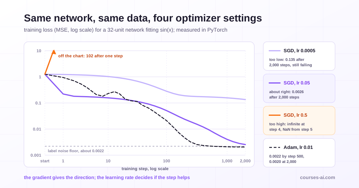
Too low, and training is stable but wasteful: after 2,000 steps the slow run is still above the loss the healthy run reached after 50. Too high, and each step overshoots by more than the last: the diverging run went from 1.257 to 102 to about 850,000 to roughly 8 x 10^17 in three steps. A loss that turns into NaN usually means a learning rate that is too high or a gradient that exploded.
Gradient clipping (torch.nn.utils.clip_grad_norm_) prevented the overflow but not the erratic loss, which kept oscillating between about 0.13 and 0.30 to the end: a guardrail against occasional spikes, common in Transformer training, not a substitute for a sensible learning rate. Sweep it in powers of ten first, and use a schedule (warmup, then decay) for long runs.
Vanishing and exploding gradients
The gradient for an early weight is a product of local derivatives from every layer above it. If those factors are mostly below one, the product shrinks exponentially with depth; if mostly above one, it grows. To see it, build a 20-layer network of 64-unit layers, run one backward pass and compare gradient sizes at the first and last layers:
import torch
from torch import nn

def grad_norms(activation, he_init=False, depth=20):
    torch.manual_seed(0)
    layers = []
    for _ in range(depth):
        linear = nn.Linear(64, 64)
        if he_init:
            nn.init.kaiming_normal_(linear.weight, nonlinearity="relu")
            nn.init.zeros_(linear.bias)
        layers += [linear, activation()]
    model = nn.Sequential(*layers, nn.Linear(64, 1))
    x = torch.randn(128, 64)
    model(x).pow(2).mean().backward()
    return model[0].weight.grad.norm().item(), model[-1].weight.grad.norm().item()

for name, act, he in [("sigmoid, default init", nn.Sigmoid, False),
                      ("relu, default init", nn.ReLU, False),
                      ("relu, He init", nn.ReLU, True)]:
    first, last = grad_norms(act, he)
    print(f"{name:22s} first layer {first:.1e}   last layer {last:.1e}")
Output:
sigmoid, default init  first layer 9.5e-19   last layer 5.8e-01
relu, default init     first layer 4.2e-10   last layer 9.2e-03
relu, He init          first layer 8.2e-02   last layer 7.7e-01
With sigmoid activations the first layer gets about 10^-18 of the last layer's gradient and will never move: the sigmoid's derivative is at most 0.25, and twenty such factors erase the signal. ReLU helps, but with PyTorch's default nn.Linear initialization the first-layer gradient is still around 10^-10 here. The initialization for rectifiers from He et al., Delving Deep into Rectifiers, keeps the first and last layers within an order of magnitude of each other.
ReLU-family activations, careful initialization, normalization layers and residual connections (a path that lets the gradient skip layers) all exist to keep that product near one. When a deep network stops learning, measure per-layer gradient norms first.
Overfitting: when the training loss is too good
The goal is good predictions on unseen data, not a low training loss. The sin run settled near 0.002 because its labels carry noise with a variance of about 0.0022, which no function of x can predict; a training loss far below the noise level means memorization.
To provoke it, train a much larger network (two hidden layers of 256 units, Adam at 0.01) on only 16 points whose labels carry noise with variance 0.09, and measure the loss on 512 held-out points after every step:
import torch
from torch import nn

torch.manual_seed(0)
X_train = torch.rand(16, 1) * 6 - 3
Y_train = torch.sin(X_train) + 0.3 * torch.randn_like(X_train)  # noise variance 0.09
X_val = torch.rand(512, 1) * 6 - 3
Y_val = torch.sin(X_val) + 0.3 * torch.randn_like(X_val)

model = nn.Sequential(nn.Linear(1, 256), nn.ReLU(),
                      nn.Linear(256, 256), nn.ReLU(), nn.Linear(256, 1))
optimizer = torch.optim.Adam(model.parameters(), lr=0.01)
loss_fn = nn.MSELoss()
best = (float("inf"), 0)

for step in range(1, 5001):
    loss = loss_fn(model(X_train), Y_train)
    optimizer.zero_grad()
    loss.backward()
    optimizer.step()
    with torch.no_grad():
        val = loss_fn(model(X_val), Y_val).item()
    best = min(best, (val, step))
    if step in (10, 100, 1000, 5000):
        print(f"step {step:4d}  train {loss.item():.4f}  validation {val:.4f}")

print(f"best validation {best[0]:.4f} at step {best[1]}")
Output:
step   10  train 0.2293  validation 0.5194
step  100  train 0.0169  validation 0.3504
step 1000  train 0.0036  validation 0.3637
step 5000  train 0.0009  validation 0.4636
best validation 0.2665 at step 38
The best model on unseen data appears at step 38, when the training loss (about 0.05) has just dropped below the noise level. Everything after that is memorization: training loss keeps falling to 0.0009 while validation loss climbs from 0.27 to 0.46. Checkpoints saved at round numbers would have missed the good model entirely, which is why validation is measured often. The defenses are more data, a smaller model, weight decay, dropout and early stopping: keep the checkpoint with the best validation loss, not the last one.
Why Adam is the default
Plain SGD uses one learning rate for every parameter. Adam (Kingma and Ba, ICLR 2015) keeps running averages of each parameter's gradient and squared gradient and divides each update by the square root of the second, so every parameter's step is normalized by its own gradient scale and stays roughly on the order of the learning rate, whether its gradients are large or small. The paper says its hyperparameters "typically require little tuning". In the runs above, Adam reached a lower loss in 500 steps (0.0022) than SGD at its good learning rate reached in 2,000 (0.0026).
Adam stores two extra values per parameter, which matters when memory is tight, and Transformers usually train with AdamW (Loshchilov and Hutter), which applies weight decay directly to the weights instead of mixing it into the adaptive update.
Batch size
The sin example used all 256 points per step; real training samples mini-batches, because a noisy gradient from a sample is good enough to make progress. A larger batch gives a less noisy gradient that can support a larger step, so when you change the batch size, revisit the learning rate.
A debugging checklist
- Overfit ten examples first. A correct model and loop drive the loss near zero; if not, suspect the loss, shapes or data.
- Check the initial loss. With cross-entropy over V classes, an untrained model starts near ln(V).
- NaN loss: lower the learning rate, add clipping.
- Loss barely moves: learning rate too low, a missing
optimizer.step(), or gradients not reaching early layers. - Evaluation randomly worse: a missing
model.eval().
From a toy loop to a large language model
LLM pretraining is the same loop with a different loss and a very different scale. The task is next-token prediction: given the tokens so far, output a probability for every token in the vocabulary, scored with cross-entropy against the token that actually came next. Here is that loop on a toy character-level model:
import math
import torch
from torch import nn
import torch.nn.functional as F

torch.manual_seed(0)
text = "the cat sat on the mat. the dog sat on the log. " * 20
vocab = sorted(set(text))
stoi = {ch: i for i, ch in enumerate(vocab)}
data = torch.tensor([stoi[ch] for ch in text])
V = len(vocab)

# A bigram model: embedding lookup -> logits over the next character
model = nn.Sequential(nn.Embedding(V, 32), nn.Linear(32, V))
optimizer = torch.optim.AdamW(model.parameters(), lr=1e-2)

inputs, targets = data[:-1], data[1:]          # predict token t+1 from token t
for step in range(301):
    logits = model(inputs)                     # (N, V)
    loss = F.cross_entropy(logits, targets)    # next-token loss
    optimizer.zero_grad()
    loss.backward()
    optimizer.step()
    if step % 100 == 0:
        print(f"step {step:3d}  loss {loss.item():.3f}")

print(f"vocab {V}, ln(V) = {math.log(V):.3f}")
Output:
step   0  loss 2.599
step 100  loss 0.700
step 200  loss 0.698
step 300  loss 0.697
vocab 14, ln(V) = 2.639
The starting loss of 2.599 is close to ln(14) = 2.639, the loss of a model that spreads probability evenly over 14 characters: the sanity check from the list above. The loss then stalls at 0.697 because that is the limit for any model that sees only the previous character. After a space the next letter could be c, s, o, t, m, d or l, and one character of context cannot tell them apart; the conditional entropy of the text, computed directly, is 0.6965. Going lower needs more context, which is what attention in a Transformer provides.
A production pretraining run keeps these calls and changes everything around them: a Transformer, subword tokens, AdamW with warmup and decay, gradient clipping, mixed precision and batches split across many accelerators.
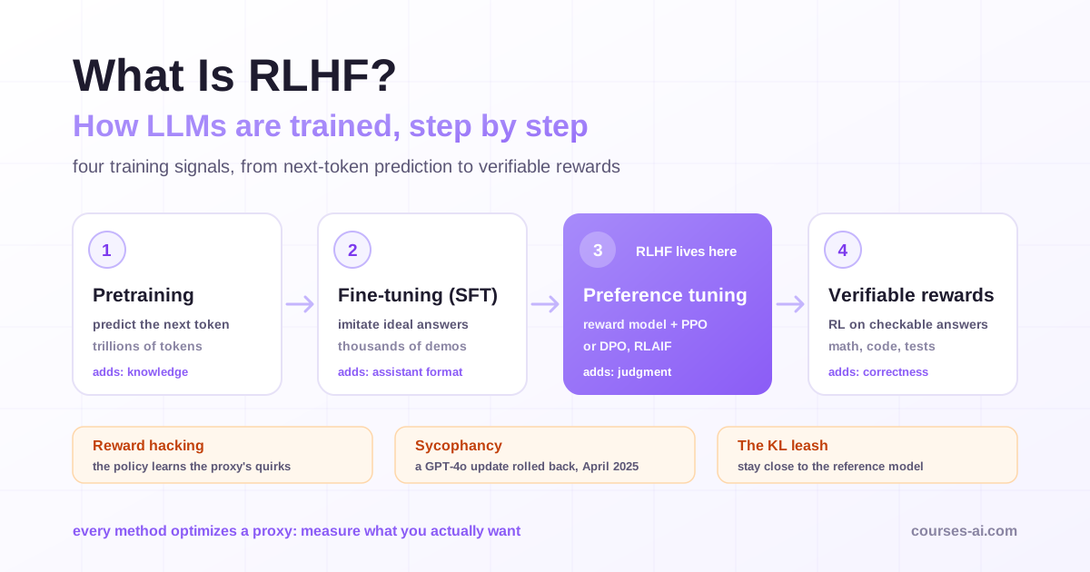
The later stages that turn a text continuer into an assistant, supervised fine-tuning and preference tuning, still run gradient descent; what changes is the data and the objective, as explained in What Is RLHF? How LLMs Are Trained. When you adapt an open-weights model yourself, LoRA freezes the original weights and trains small adapter matrices with the same loop, as in Fine-Tuning an Open-Source LLM with LoRA and QLoRA. The lessons above carry over: too high a learning rate can overwrite what the model knew, and too many epochs on a small dataset memorize it.
Where neural networks sit among LLM APIs, RAG and agents is the scope of Introduction to AI Engineering; What Is an AI Engineer? separates building with models from training them.
Frequently Asked Questions (FAQ)
How do neural networks learn, in one sentence? They repeat a loop: predict, measure the error with a loss function, use backpropagation to compute how each weight affects that error, and use gradient descent to move every weight a small step in the direction that lowers it.
What is the difference between backpropagation and gradient descent?
Backpropagation computes the gradient of the loss with respect to every parameter, using the chain rule from the output backward. Gradient descent, or an optimizer such as Adam, uses that gradient to update the parameters. In PyTorch, loss.backward() is backpropagation and optimizer.step() is the update.
How do I choose a learning rate? Try values spaced by powers of ten and watch the first few hundred steps. A loss that turns into NaN usually means too high (or a numerical bug such as log of zero); a loss that barely moves usually means too low. Around 1e-3 is the usual starting point for Adam, but only the loss curve on your problem settles it.
Do large language models learn the same way? At the level of the algorithm, yes. Pretraining is next-token prediction with a cross-entropy loss, optimized with backpropagation and, in most published training runs, an Adam-family optimizer. The architecture, data volume, hardware and later training stages differ.
Conclusion
A neural network learns by turning "how wrong was that" into one number and asking, for every parameter, which direction makes that number smaller. Backpropagation answers the direction question exactly and cheaply with the chain rule; gradient descent decides how far to move. The four-parameter example contains the whole mechanism and its main weakness: the gradient is a local slope, so the learning rate decides whether a step helps or hurts. Initialization, residual connections, Adam, validation sets and clipping exist to keep that loop stable at depth and scale.
Sources
- Learning representations by back-propagating errors, David E. Rumelhart, Geoffrey E. Hinton and Ronald J. Williams, Nature 323, 533-536, 9 October 1986
- Deep Learning, chapter 6: Deep Feedforward Networks, Ian Goodfellow, Yoshua Bengio and Aaron Courville, MIT Press, 2016 (section 6.5 and the historical notes in section 6.6)
- Optimizing Model Parameters, PyTorch tutorials
- Adam: A Method for Stochastic Optimization, Diederik P. Kingma and Jimmy Ba, arXiv:1412.6980, ICLR 2015
- Delving Deep into Rectifiers, Kaiming He, Xiangyu Zhang, Shaoqing Ren and Jian Sun, arXiv:1502.01852, 2015
- Also cited: Loshchilov and Hutter, "Decoupled Weight Decay Regularization" (AdamW), arXiv:1711.05101; PyTorch documentation for
torch.optim.Optimizer.zero_grad
Verified on 10 November 2026 against the sources above; every code block was run on PyTorch 2.8.0 (CPU) with Python 3.9, and the outputs shown are the actual outputs.

The course that continues this article
Deep Learning and Neural Networks with PyTorch
You have read the theory. In the course you put it into practice: written lessons structured in modules, with examples and exercises, quizzes, the AI Professor in every lesson and progress saved automatically. Once you complete the lessons and reach the minimum quiz score, you get the Certificate of Completion, a private attestation.
From the course syllabus
- Foundations: Why Deep Learning in 2026
- PyTorch Tensors and Autograd
- From Linear Regression to Neural Networks
- Backpropagation and Gradient Descent
+ 8 more modules in the full syllabus
€99 per month for this course, VAT included · or pick it in a subscription of 3, 5 or 10 courses, from €199 per month, together with other IT courses; you can change them at every renewal (see what you learn across the whole track).
Monthly subscription with automatic renewal · stop the renewal anytime from your account · digital content with immediate access, see the withdrawal conditions. The certificate confirms that you completed the course and is private: it is not a diploma or a state-recognised qualification.